共通資料: Plots: Basic & Common Attributes 基礎&属性
1. Plots について
Julia programming におけるグラフの作成によく使われている外部 Package である。
公式 Tutorial はこちら
グラフの指令を実行する前に、一度次の指令を実行しないといけないです。
using Plots
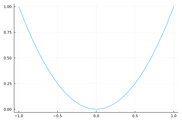
2. plot で曲線を描く
plot 始めの例
using Plots
x = -1:0 .1:1
y = x.^2
plot(x, y)
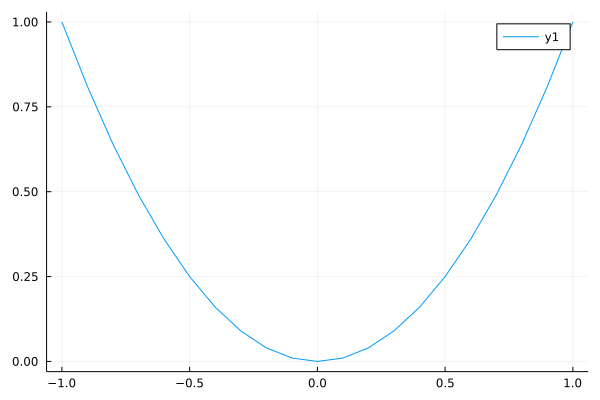
Legend を無効にする
x = -1:0 .1:1
y = x.^2
plot(x, y, legend = false)
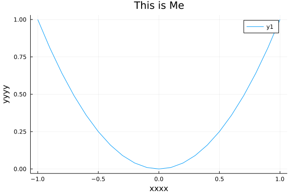
3. 属性:軸ラベルとタイトル
グラフのスタイル、曲線の色、太さなどの情報(データ、引数等)は
文法は次通り:
plot(x,y, ある属性 = その値
軸ラベルとタイトルの属性を指定する例
次の属性を指定して軸にラベルとタイトルを編集する
►
►
►
x = -1:0 .1:1
y = x.^2
plot(x, y, xlabel = "xxxx" , ylabel = "yyyy" , title = "This is Me" )
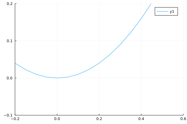
4. 属性:グラフ範囲
次の属性で曲線を描く範囲を指定する。
►
►
x = -1:0 .05:1
y = x.^2
plot(x, y, xlims = (-0.2 , 0.6 ), ylims = (-0.1 , 0.2 ))
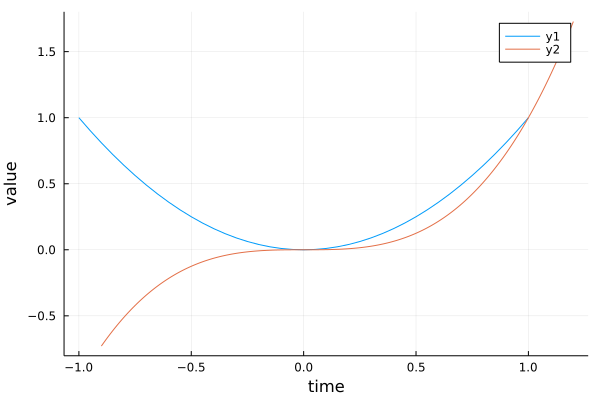
5. plot!で曲線を追加
例1:グラフ範囲:自動
t1 = -1:0 .05:1
y1 = t1.^2
t2 = -0.9 :0.01 :1.2
y2 = t2.^3
plot(t1, y1, xlabel = "time" , ylabel = "value" )
plot!(t2, y2) #同じグラフに 曲線を追加する
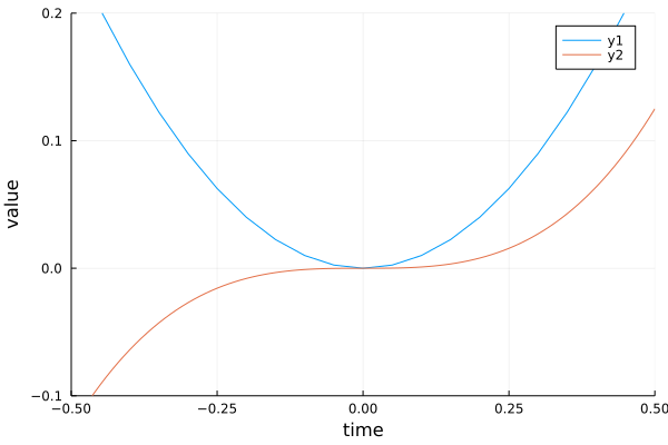
例2:グラフ範囲:指定
t1 = -1:0 .05:1
y1 = t1.^2
t2 = -0.9 :0.01 :1.2
y2 = t2.^3
plot(t1, y1, xlabel = "time" , ylabel = "value" )
plot!(t2, y2) #同じグラフに 曲線を追加する
plot!(xlims = (-0.5 , 0.5 ), ylims = (-0.1 , 0.2 )) #範囲指定の設定を追加する
6. 属性:色、太さ、グラフサイズ
► 省略:
► 例: :red, :blue
► 省略:
► 線の太さ、単位は point pt
► 省略:
► 例: :auto, :solid, :dash, :dot, :dashdot, :dashdotdot
x = 0:0 .01:1
plot(x, x.^1 , color = :red)#色:青、その他は指定しない
plot!(x, x.^0.5 , linecolor=:blue, linestyle = :dot, linewidth = 2 ,)#色:赤、点線、太さ= 2
plot!(x, x.^2 , lc=:green, ls = :dash, lw = 3 )#色:緑、破線、太さ= 3
plot!( size = (400,400 ) ) #グラフのサイズを指定する

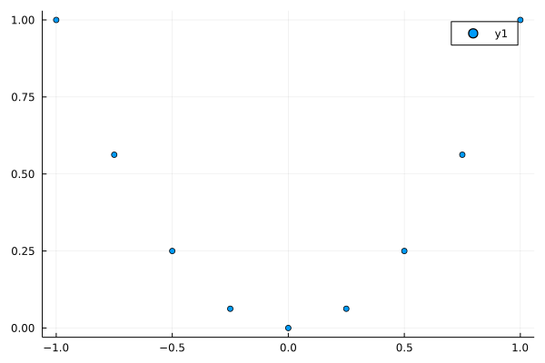
7. scatter で散乱図を描く
デフォルト例
x = -1:0 .25:1
y = x .^2
scatter(x, y)
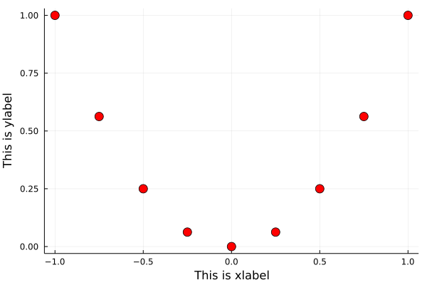
Attribute 属性を指定する例
x = -1:0 .25:1
y = x .^2
scatter(x, y,
xlabel = "This is xlabel" , #軸ラベルの属性は plot と同じ
ylabel = "This is ylabel" ,
marker = 7 , #点のサイズ
color = :red, #点の色
legend = false
)
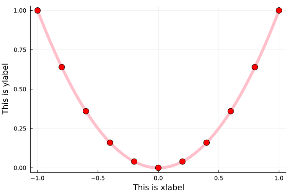
8. scatter! で散乱図を追加
plot! と同じ、scatter! を使ってグラフに散乱図を追加することができる。
x = -1:0 .2:1 #散乱図用
y = x .^2
a = -1:0 .01:1 #曲線用
b = a.^2
plot(a, b, color = :pink, linewidth = 6 ) #曲線を先に描く
scatter!(x, y,
xlabel = "This is xlabel" , #軸ラベルの属性は plot と同じ
ylabel = "This is ylabel" ,
marker = 7 , #点のサイズ
color = :red, #点の色
legend = false
)
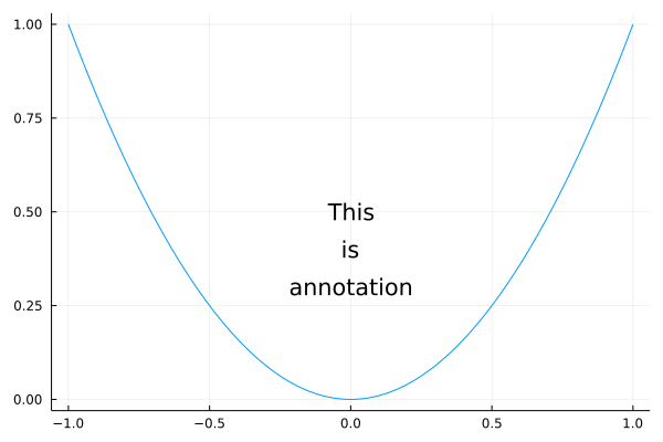
9. 属性:annotation で注釈を追加
a = -1:0 .01:1
b = a.^2
plot(a, b, legend = false)
plot!(annotation = (0 , 0.5 , "This" )) #注釈 を追加する
plot!(annotation = (0 , 0.4 , "is" ))
plot!(annotation = (0 , 0.3 , "annotation" ))
10. 属性 layout でグラフの配置を指定する
文法
p1 = plot(...)
p2 = plot(...)
p3 = plot(...)
plot(p1, p2, p3, layout = ...)
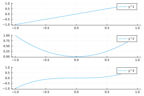
例:(3 × 1)
x = -1:0 .01:1
y1 = x.^1
y2 = x.^2
y3 = x.^3
P1 = plot(x, y1, label = "y^1" )
P2 = plot(x, y2, label = "y^2" )
P3 = plot(x, y3, label = "y^3" )
plot(P1, P2, P3, layout=(3,1 ))
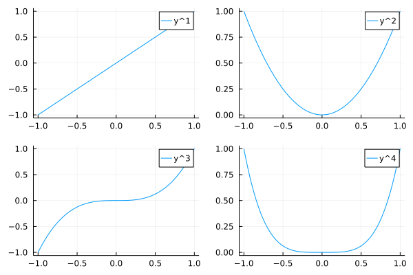
例:(2 × 2)
x = -1:0 .01:1
y1 = x.^1
y2 = x.^2
y3 = x.^3
y4 = x.^4
P1 = plot(x, y1, label = "y^1" )
P2 = plot(x, y2, label = "y^2" )
P3 = plot(x, y3, label = "y^3" )
P4 = plot(x, y4, label = "y^4" )
plot(P1, P2, P3, P4, layout=(2,2 ))
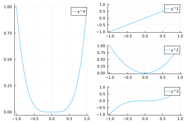
例:(3 × 1)&(1 × 2)
x = -1:0 .01:1
y1 = x.^1
y2 = x.^2
y3 = x.^3
y4 = x.^4
P1 = plot(x, y1, label = "y^1" )
P2 = plot(x, y2, label = "y^2" )
P3 = plot(x, y3, label = "y^3" )
P4 = plot(x, y4, label = "y^4" )
Q = plot(P1, P2, P3, layout=(3,1 ))
plot(P4, Q, layout=(1,2 ))
11. histogram でヒストグラムを作成
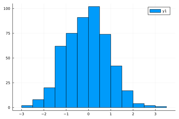
bin 指定なしの例
x = randn(500 )#標準正規分布のランダム列(500個)
histogram(x)
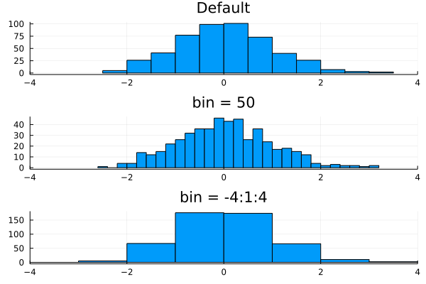
bin を指定する例
x = randn(500 )#標準正規分布のランダム列(500個)
P1 = histogram(x, title = "Default" ) # bin は指定なし -> 自動
P2 = histogram(x, bin = 50 , title = "bin = 50" )
P3 = histogram(x, bin=-4:1 :4 , title = "bin = -4:1:4" )
plot(P1, P2, P3, layout = (3,1 ), xlims = (-4,4 ), legend = false)
12. その他:軸の目盛り等
軸の目盛りは次の属性で指定できる
►
►
• 使い方1:
• 使い方2:
目盛りの方向
►
►
►
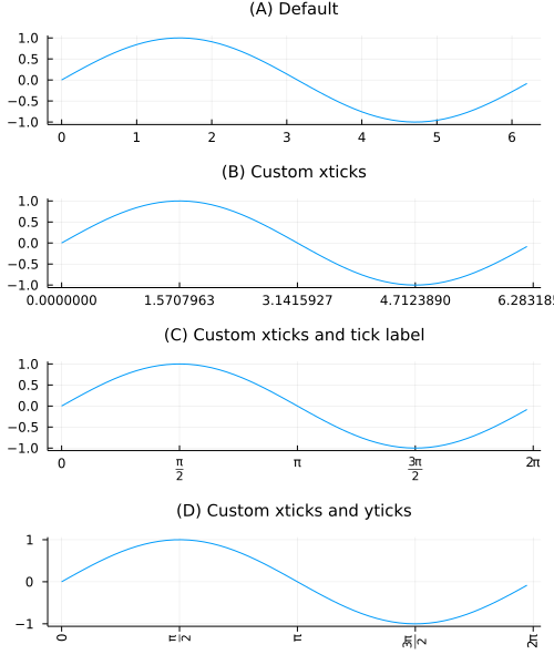
正弦波の例
x = 0:0 .1 : 2 *pi
y = sin.(x)
A = plot(x, y, legend = false, title = "(A) Default" ) #これはデフォルト設定
B = plot(x,y, legend = false, title = "(B) Custom xticks" ,
xticks = [0 , pi/2 , pi, 3 *pi/2 , 2 *pi], #手動で xticks を指定する
)
C = plot(x,y, legend = false, title = "(C) Custom xticks and tick label" ,
##手動で xticks と 目盛りラベルを指定する.
xticks =([0 , pi/2 , pi, 3 *pi/2 , 2 *pi], ["0" , "\pi/2" , "\pi" , "3\pi/2" , "2\pi" ]),
)
D = plot(x,y, legend = false, title = "(D) Custom xticks and yticks" ,
##手動で xticks と yticks を指定する.
xticks =([0 , pi/2 , pi, 3 *pi/2 , 2 *pi], ["0" , "\pi/2" , "\pi" , "3\pi/2" , "2\pi" ]),
yticks =[-1 , 0 , 1 ],
xrotation = 90 , # 文字を 90度回転
xtick_direction = :out, #x tickの方向:外向き
ytick_direction = :out, #y tickの方向:外向き
)
plot(A, B, C, D, layout = (4,1 ), titlefontsize = 10 , size = (500,600 ))
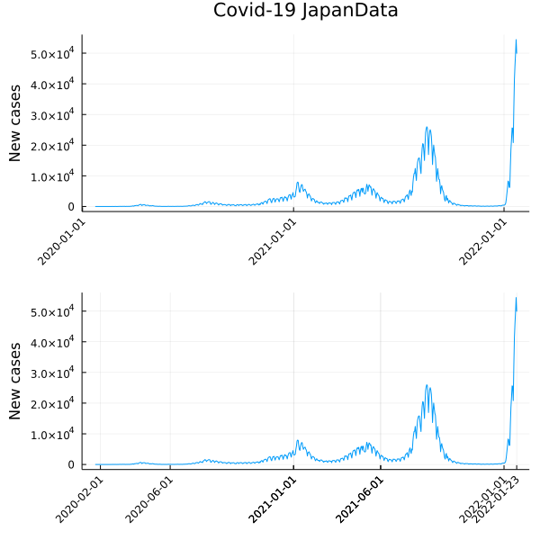
コロナ感染データの日付け(Date) を用いた例
データのリンク:owid-covid-data.csv
using Plots
using DataFrames
using CSV
using Dates
Y = CSV.read("owid-covid-data.csv" , DataFrame)
JapanData = Y[Y.location .== "Japan" , :]
#デフォルトの設定
A = plot(JapanData.date, JapanData.new_cases, legend = false,
ylabel = "New cases" ,
xrotation = 45 , title = "Covid-19 JapanData" )
#手動で横軸(日付け)の目盛りを指定する
B = plot(JapanData.date, JapanData.new_cases, legend = false,
ylabel = "New cases" ,
xticks = [
Date(2020,2 ,1 ), Date(2020,6 ,1 ),
Date(2021,1 ,1 ), Date(2021,6 ,1 ),
Date(2022,1 ,1 ), Date(2022,1 ,23 )
],
xrotation = 45
)
plot(A,B,layout = (2,1 ), size = (600,600 ))
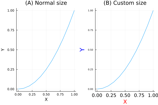
13. その他:軸のフォントサイズ
軸のフォントサイズは次の属性で指定できる
►
►
►
►
x = 0:0 .1 : 1
y = x.^2
A = plot(x,y, legend = false, title = "(A) Normal size" ,
xlabel = "X" , ylabel = "Y"
)
B = plot(x,y, legend = false, title = "(B) Custom size" ,
xlabel = "X" , ylabel = "Y" ,
xtickfontsize = 12 , #目盛りのフォントサイズ
ytickfontsize = 6 ,
ylabelfontsize = 16 , #軸ラベルのフォントサイズ
xlabelfontsize = 14 ,
xguidefontcolor = :red, #軸ラベルの色
yguidefontcolor = :blue
)
plot(A, B, layout = (1,2 ))